Performing Spatial Queries

Introduction

Spatial queries allows you to select features in a layer by their spatial relationships with features from another layer. GeoPandas provides sjoin() and sjoin_nearest() functions that can be used to perform a spatial query.

Overview of the Task

We will be working with 2 data layers for the city of Melbourne, Australia. Given the data layers for the pubs and bars in the city and the locations of all metro stations, we want to find out which bars and pubs are within 500 meters of a metro station.

Input Layers:

• metro_stations_accessbility.zip: A shapefile of metro stations in Melbourne

• Bars_and_pubs__with_patron_capacity.csv: CSV file with location of bars and pubs in Melbournse

Output:

• spatial_query.gpkg: A GeoPackage containing all bars and pubs within 500 meters of a metro station

Data Credit

• 2019 The City of Melbourne Open Data Portal. Data provided by Metro Trains Melbourne and Census of Land Use and Employment (CLUE)

Watch Video Walkthrough

Setup and Data Download

The following blocks of code will install the required packages and download the datasets to your Colab environment.

import os
import pandas as pd
import geopandas as gpd
import matplotlib.pyplot as plt

data_folder = 'data'
output_folder = 'output'

if not os.path.exists(data_folder):
    os.mkdir(data_folder)
if not os.path.exists(output_folder):
    os.mkdir(output_folder)

def download(url):
    filename = os.path.join(data_folder, os.path.basename(url))
    if not os.path.exists(filename):
        from urllib.request import urlretrieve
        local, _ = urlretrieve(url, filename)
        print('Downloaded ' + local)

data_url = 'https://github.com/spatialthoughts/geopython-tutorials/releases/download/data/'

download(data_url + 'Bars_and_pubs__with_patron_capacity.csv')
download(data_url + 'metro_stations_accessbility.zip')

Downloaded data/Bars_and_pubs__with_patron_capacity.csv
Downloaded data/metro_stations_accessbility.zip

Procedure

Read the Bars_and_pubs__with_patron_capacity.csv file and convert it to a GeoDataFrame.

csv_file = 'Bars_and_pubs__with_patron_capacity.csv'
csv_path = os.path.join(data_folder, csv_file)
barspubs_df = pd.read_csv(csv_path) 
barspubs_df.iloc[:, :5]

	Census year	Block ID	Property ID	Base property ID	Street address
0	2002	247	106238	106238	192-202 Lygon Street
1	2002	252	106244	106244	160-162 Lygon Street
2	2006	16	104018	104018	172-192 Flinders Street
3	2002	214	106186	106186	414-422 Lygon Street
4	2008	76	589841	105749	221 Little Lonsdale Street
...	...	...	...	...	...
3333	2017	85	105746	105746	183-265 La Trobe Street
3334	2017	74	104662	104662	106-112 Hardware Street
3335	2017	268	108154	108153	49 Rathdowne Street
3336	2017	104	104085	104085	167-175 Franklin Street
3337	2017	33	100730	100730	12-16 Bank Place

3338 rows × 5 columns

You will note that the data contains multiple features for each establishment from different years. Let’s sort by Property ID and check.

barspubs_df = barspubs_df.sort_values('Property ID')
barspubs_df.iloc[:, :5]

	Census year	Block ID	Property ID	Base property ID	Street address
3129	2017	103	100160	100160	196-200 A'Beckett Street
709	2011	103	100160	100160	196-200 A'Beckett Street
2553	2015	103	100160	100160	196-200 A'Beckett Street
247	2008	103	100160	100160	196-200 A'Beckett Street
2201	2010	103	100160	100160	196-200 A'Beckett Street
...	...	...	...	...	...
2579	2015	1105	628712	628712	717-731 Collins Street
2832	2016	66	635138	635138	13 Heffernan Lane
3069	2017	66	635138	635138	13 Heffernan Lane
3058	2016	270	664626	104468	230 Grattan Street
3228	2017	270	664626	104468	230 Grattan Street

3338 rows × 5 columns

We are interested only in the location of the establishment. So we can de-duplicate the dataframe and keep only 1 record per unique Property ID.

barspubs_df = barspubs_df.drop_duplicates(subset=['Property ID'], keep='first')
barspubs_df.iloc[:, :5]

	Census year	Block ID	Property ID	Base property ID	Street address
3129	2017	103	100160	100160	196-200 A'Beckett Street
1087	2011	409	100441	100441	118-126 Ireland Street
410	2004	315	100514	100514	204-206 Arden Street
1501	2009	33	100727	100727	5-9 Bank Place
1159	2013	33	100730	100730	12-16 Bank Place
...	...	...	...	...	...
1601	2009	2391	616966	616966	2 Boundary Road
1182	2013	1110	620312	593737	23-37 Star Crescent
3028	2016	1105	628712	628712	717-731 Collins Street
2832	2016	66	635138	635138	13 Heffernan Lane
3058	2016	270	664626	104468	230 Grattan Street

308 rows × 5 columns

Now that we are done with data cleaning, let’s turn this dataframe in to a spatial layer. The location of the establishment is defined using the x coordinate and y coordinate columns.

barspubs_df.iloc[:, -5:]

	Trading name	Number of patrons	x coordinate	y coordinate	Location
3129	Nomads Industry Backpackers	200	144.957445	-37.809985	(-37.80998494, 144.9574447)
1087	Railway Hotel	241	144.942118	-37.806054	(-37.80605366, 144.9421177)
410	North Melbourne Football Club Social Club	210	144.941312	-37.799055	(-37.79905531, 144.9413118)
1501	Mitre Tavern	300	144.960311	-37.816805	(-37.81680457, 144.9603112)
1159	Melbourne Savage Club	90	144.960577	-37.816545	(-37.81654467, 144.9605765)
...	...	...	...	...	...
1601	Vodka Locka & Red Leaf Restaurant	40	144.939233	-37.795318	(-37.79531826, 144.9392333)
1182	Harbour Town Hotel	498	144.937830	-37.813150	(-37.81315031, 144.9378299)
3028	Bar Nicional	75	144.950093	-37.820687	(-37.82068699, 144.9500934)
2832	Union Electric	72	144.966591	-37.811802	(-37.81180178, 144.9665913)
3058	HJC Bar	200	144.961247	-37.797398	(-37.79739836, 144.9612468)

308 rows × 5 columns

Create a geometry column and use it to define a new GeoDataFrame.

geometry = gpd.points_from_xy(barspubs_df['x coordinate'],barspubs_df['y coordinate'])
barspubs_gdf = gpd.GeoDataFrame(barspubs_df, crs='EPSG:4326', geometry=geometry)

Next, we will read the zipped shapefile of metro stations as a GeoDataFrame.

zip_file = 'metro_stations_accessbility.zip'
zip_path = os.path.join('zip://', data_folder, zip_file)
metrostations_gdf = gpd.read_file(zip_path)
metrostations_gdf

	station	pids	he_loop	lift	geometry
0	Alamein	No	No	No	POINT (145.07956 -37.86884)
1	Albion	Dot Matrix	No	No	POINT (144.82471 -37.77766)
2	Alphington	Dot Matrix	No	No	POINT (145.03125 -37.7784)
3	Altona	LCD	No	No	POINT (144.8306 -37.86725)
4	Anstey	No	No	No	POINT (144.96056 -37.7619)
...	...	...	...	...	...
214	Williams Landing	Dot Matrix	Yes	Yes	POINT (144.74719 -37.8701)
215	Aircraft	No	No	No	POINT (144.76081 -37.8666)
216	Flemington Racecourse	No	No	No	POINT (144.9072 -37.78759)
217	Showgrounds	No	No	No	POINT (144.91498 -37.78355)
218	Southland	LCD	Yes	Yes	POINT (145.04867 -37.95818)

219 rows × 5 columns

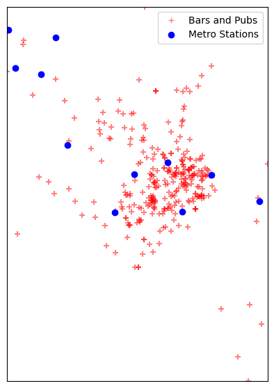
Visualize the layers.

fig, ax = plt.subplots(1, 1)
fig.set_size_inches(15,7)
barspubs_gdf.plot(ax=ax, color='red', alpha=0.5, marker='+')
metrostations_gdf.plot(ax=ax, color='blue', alpha=1, marker='o')

minx, miny, maxx, maxy = barspubs_gdf.total_bounds
ax.set_xlim(minx, maxx)
ax.set_ylim(miny, maxy)

legend_elements = [
    plt.plot([],[], color='red', alpha=0.5, marker='+', label='Bars and Pubs', ls='')[0],
    plt.plot([],[], color='blue', alpha=1, marker='o', label='Metro Stations', ls='')[0]]
ax.legend(handles=legend_elements, loc='upper right')
ax.get_xaxis().set_visible(False)
ax.get_yaxis().set_visible(False)
plt.show()

For performing any analysis, we must use a Projected CRS. Let’s reproject to a local CRS for Melbourne. GDA 2020 / MGA zone 55 EPSG:7855.

metrostations_gdf_reprojected = metrostations_gdf.to_crs('EPSG:7855')
barspubs_gdf_reprojected = barspubs_gdf.to_crs('EPSG:7855')

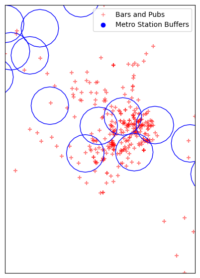
We now buffer the metro stations to 500 meters. GeoPandas uses shapely for buffer operation. We specify buffer parameters to match QGIS’s default style.

radius = 500

buffer_geometry = metrostations_gdf_reprojected.buffer(
    radius, resolution=5, cap_style=1, join_style=1, mitre_limit=2)
metrostations_gdf_reprojected['geometry'] = buffer_geometry

Visualize the buffers.

fig, ax = plt.subplots(1, 1)
fig.set_size_inches(15,7)
barspubs_gdf_reprojected.plot(ax=ax, color='red', alpha=0.5, marker='+')
metrostations_gdf_reprojected.plot(ax=ax, facecolor='none', edgecolor='blue',  alpha=1, marker='o')

minx, miny, maxx, maxy = barspubs_gdf_reprojected.total_bounds
ax.set_xlim(minx, maxx)
ax.set_ylim(miny, maxy)

legend_elements = [
    plt.plot([],[], color='red', alpha=0.5, marker='+', label='Bars and Pubs', ls='')[0],
    plt.plot([],[], color='blue', alpha=1, marker='o', label='Metro Station Buffers', ls='')[0]]
ax.legend(handles=legend_elements, loc='upper right')
ax.get_xaxis().set_visible(False)
ax.get_yaxis().set_visible(False)
plt.show()

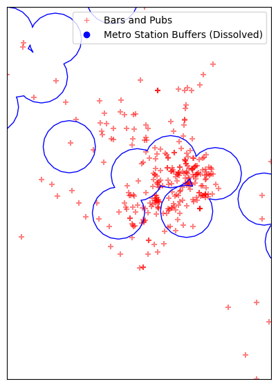
As we want to do a spatial join, we need to dissolve the resulting buffers. Otherwise we will get 1 feature for every intersecting buffer

metrostations_gdf_reprojected['dissolvefield'] = 1
dissolved_buffers = metrostations_gdf_reprojected.dissolve(by='dissolvefield')

fig, ax = plt.subplots(1, 1)
fig.set_size_inches(15,7)
barspubs_gdf_reprojected.plot(ax=ax, color='red', alpha=0.5, marker='+')
dissolved_buffers.plot(ax=ax, facecolor='none', edgecolor='blue',  alpha=1)

minx, miny, maxx, maxy = barspubs_gdf_reprojected.total_bounds
ax.set_xlim(minx, maxx)
ax.set_ylim(miny, maxy)

legend_elements = [
    plt.plot([],[], color='red', alpha=0.5, marker='+', label='Bars and Pubs', ls='')[0],
    plt.plot([],[], color='blue', alpha=1, marker='o', label='Metro Station Buffers (Dissolved)', ls='')[0]]
ax.legend(handles=legend_elements, loc='upper right')
ax.get_xaxis().set_visible(False)
ax.get_yaxis().set_visible(False)
plt.show()

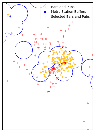
Now do a spatial join to select all bars and pubs within the dissolved buffer region.

selected = barspubs_gdf_reprojected.sjoin(
    dissolved_buffers, how='inner', predicate='within')

For our final visualization, we show the selected establishments within the buffer zone.

fig, ax = plt.subplots(1, 1)
fig.set_size_inches(15,7)
barspubs_gdf_reprojected.plot(ax=ax, color='red', alpha=0.5, marker='+')
dissolved_buffers.plot(ax=ax, facecolor='none', edgecolor='blue',  alpha=1)
selected.plot(ax=ax, color='yellow', alpha=0.5, marker='+')

minx, miny, maxx, maxy = barspubs_gdf_reprojected.total_bounds
ax.set_xlim(minx, maxx)
ax.set_ylim(miny, maxy)

legend_elements = [
    plt.plot([],[], color='red', alpha=0.5, marker='+', label='Bars and Pubs', ls='')[0],
    plt.plot([],[], color='blue', alpha=1, marker='o', label='Metro Station Buffers', ls='')[0],
    plt.plot([],[], color='yellow', alpha=1, marker='+', label='Selected Bars and Pubs', ls='')[0]
]

ax.legend(handles=legend_elements, loc='upper right')
ax.get_xaxis().set_visible(False)
ax.get_yaxis().set_visible(False)

plt.show()

Finally, we save all our layers into a output geopackage.

output_file = 'spatial_query.gpkg'
output_path = os.path.join(output_folder, output_file)

barspubs_gdf_reprojected.to_file(filename=output_path, layer='bars_and_pubs')
metrostations_gdf_reprojected.to_file(filename=output_path, layer='metro_stations')
selected.to_file(filename=output_path, layer='selected_locations')

---

If you want to give feedback or share your experience with this tutorial, please comment below. (requires GitHub account)