Transform Longitude Values

Introduction

Many climate datasets have longitude coordinates from 0 to 360. This is not suitable to be used in other raster based geoprocessing systems. This notebook shows how to convert such datasets to span longitude from -180 to +180 and save it as a GeoTIFF file suitable for analysis in GIS software.

Overview of the Task

We take a NetCDF file of Monthly Precipitation by ECMWF ERA5-Land Monthly Average dataset. This file has global monthly precipitation for the month of July, 2021. We reproject the longitude coordinates and save the result as a GeoTIFF file.

Input Layers:

• era5-land-precipitation.nc: A NetCDF file containing monthly average precipitation with longitude coordinates from 0-360.

Output:

• precipitation.tif: A reprojected GeoTiff file of total monthly precpitation with longitudes from -180 to +180.

Data Credit:

• Muñoz Sabater, J., (2019): ERA5-Land monthly averaged data from 1981 to present. Copernicus Climate Change Service (C3S) Climate Data Store (CDS). (Accessed on < 05-Aug-2022 >), 10.24381/cds.68d2bb3

Setup and Data Download

The following blocks of code will install the required packages and download the datasets to your Colab environment.

%%capture
if 'google.colab' in str(get_ipython()):
    !pip install rioxarray netcdf4 cartopy

import cartopy.crs as ccrs
import matplotlib.pyplot as plt
import os
import pandas as pd
import rioxarray as rxr
import xarray as xr

data_folder = 'data'
output_folder = 'output'

if not os.path.exists(data_folder):
    os.mkdir(data_folder)
if not os.path.exists(output_folder):
    os.mkdir(output_folder)

def download(url):
    filename = os.path.join(data_folder, os.path.basename(url))
    if not os.path.exists(filename):
        from urllib.request import urlretrieve
        local, _ = urlretrieve(url, filename)
        print('Downloaded ' + local)

filename = 'era5-land-precipitation.nc'
data_url = 'https://github.com/spatialthoughts/geopython-tutorials/releases/download/data/'

download(data_url + filename)

Procedure

Open the input file with XArray.

input_path = os.path.join(data_folder, filename)
ds = xr.open_dataset(input_path)
ds

<xarray.Dataset> Size: 52MB
Dimensions:    (longitude: 3600, latitude: 1801, time: 1)
Coordinates:
  * longitude  (longitude) float32 14kB 0.0 0.1 0.2 0.3 ... 359.7 359.8 359.9
  * latitude   (latitude) float32 7kB 90.0 89.9 89.8 89.7 ... -89.8 -89.9 -90.0
  * time       (time) datetime64[ns] 8B 2021-07-01
Data variables:
    tp         (time, latitude, longitude) float64 52MB ...
Attributes:
    Conventions:  CF-1.6
    history:      2022-08-05 17:45:55 GMT by grib_to_netcdf-2.25.1: /opt/ecmw...

xarray.Dataset

• Dimensions:
  • longitude: 3600
  • latitude: 1801
  • time: 1
• Coordinates: (3)
  • longitude
    (longitude)
    float32
    0.0 0.1 0.2 ... 359.7 359.8 359.9

    units :

    degrees_east

    long_name :

    longitude

    array([0.000e+00, 1.000e-01, 2.000e-01, ..., 3.597e+02, 3.598e+02, 3.599e+02],
          dtype=float32)

  • latitude
    (latitude)
    float32
    90.0 89.9 89.8 ... -89.9 -90.0

    units :

    degrees_north

    long_name :

    latitude

    array([ 90. ,  89.9,  89.8, ..., -89.8, -89.9, -90. ], dtype=float32)

  • time
    (time)
    datetime64[ns]
    2021-07-01

    long_name :

    time

    array(['2021-07-01T00:00:00.000000000'], dtype='datetime64[ns]')

• Data variables: (1)
  • tp
    (time, latitude, longitude)
    float64
    ...

    units :

    m

    long_name :

    Total precipitation

    [6483600 values with dtype=float64]

• Indexes: (3)
  • longitude
    PandasIndex

    PandasIndex(Index([                0.0, 0.10000000149011612, 0.20000000298023224,
           0.30000001192092896,  0.4000000059604645,                 0.5,
            0.6000000238418579,   0.699999988079071,   0.800000011920929,
            0.8999999761581421,
           ...
                         359.0,   359.1000061035156,  359.20001220703125,
            359.29998779296875,   359.3999938964844,               359.5,
             359.6000061035156,  359.70001220703125,  359.79998779296875,
             359.8999938964844],
          dtype='float32', name='longitude', length=3600))

  • latitude
    PandasIndex

    PandasIndex(Index([              90.0,   89.9000015258789,  89.80000305175781,
            89.69999694824219,   89.5999984741211,               89.5,
             89.4000015258789,  89.30000305175781,  89.19999694824219,
             89.0999984741211,
           ...
            -89.0999984741211, -89.19999694824219, -89.30000305175781,
            -89.4000015258789,              -89.5,  -89.5999984741211,
           -89.69999694824219, -89.80000305175781,  -89.9000015258789,
                        -90.0],
          dtype='float32', name='latitude', length=1801))

  • time
    PandasIndex

    PandasIndex(DatetimeIndex(['2021-07-01'], dtype='datetime64[ns]', name='time', freq=None))

• Attributes: (2)

  Conventions :

  CF-1.6

  history :

  2022-08-05 17:45:55 GMT by grib_to_netcdf-2.25.1: /opt/ecmwf/mars-client/bin/grib_to_netcdf.bin -S param -o /cache/data2/adaptor.mars.internal-1659721554.6110172-11067-16-54c3e992-66c1-41ea-b6a9-bd330d7a50d7.nc /cache/tmp/54c3e992-66c1-41ea-b6a9-bd330d7a50d7-adaptor.mars.internal-1659721554.07149-11067-24-tmp.grib

Notice the longitude coordinates have have values from 0 to 360. We convert the longitude to range from -180 to +180. Many downstream packages expect the coordinates to be sorted in ascening order, so we also sort the resulting longitude values.

ds.coords['longitude'] = (ds.coords['longitude'] + 180) % 360 - 180
ds = ds.sortby(ds.longitude)
ds

<xarray.Dataset> Size: 52MB
Dimensions:    (latitude: 1801, time: 1, longitude: 3600)
Coordinates:
  * latitude   (latitude) float32 7kB 90.0 89.9 89.8 89.7 ... -89.8 -89.9 -90.0
  * time       (time) datetime64[ns] 8B 2021-07-01
  * longitude  (longitude) float32 14kB -180.0 -179.9 -179.8 ... 179.8 179.9
Data variables:
    tp         (time, latitude, longitude) float64 52MB ...
Attributes:
    Conventions:  CF-1.6
    history:      2022-08-05 17:45:55 GMT by grib_to_netcdf-2.25.1: /opt/ecmw...

xarray.Dataset

• Dimensions:
  • latitude: 1801
  • time: 1
  • longitude: 3600
• Coordinates: (3)
  • latitude
    (latitude)
    float32
    90.0 89.9 89.8 ... -89.9 -90.0

    units :

    degrees_north

    long_name :

    latitude

    array([ 90. ,  89.9,  89.8, ..., -89.8, -89.9, -90. ], dtype=float32)

  • time
    (time)
    datetime64[ns]
    2021-07-01

    long_name :

    time

    array(['2021-07-01T00:00:00.000000000'], dtype='datetime64[ns]')

  • longitude
    (longitude)
    float32
    -180.0 -179.9 ... 179.8 179.9

    array([-180.     , -179.9    , -179.79999, ...,  179.70001,  179.79999,
            179.9    ], dtype=float32)

• Data variables: (1)
  • tp
    (time, latitude, longitude)
    float64
    ...

    units :

    m

    long_name :

    Total precipitation

    [6483600 values with dtype=float64]

• Indexes: (3)
  • latitude
    PandasIndex

    PandasIndex(Index([              90.0,   89.9000015258789,  89.80000305175781,
            89.69999694824219,   89.5999984741211,               89.5,
             89.4000015258789,  89.30000305175781,  89.19999694824219,
             89.0999984741211,
           ...
            -89.0999984741211, -89.19999694824219, -89.30000305175781,
            -89.4000015258789,              -89.5,  -89.5999984741211,
           -89.69999694824219, -89.80000305175781,  -89.9000015258789,
                        -90.0],
          dtype='float32', name='latitude', length=1801))

  • time
    PandasIndex

    PandasIndex(DatetimeIndex(['2021-07-01'], dtype='datetime64[ns]', name='time', freq=None))

  • longitude
    PandasIndex

    PandasIndex(Index([             -180.0, -179.89999389648438, -179.79998779296875,
           -179.70001220703125, -179.60000610351562,              -179.5,
           -179.39999389648438, -179.29998779296875, -179.20001220703125,
           -179.10000610351562,
           ...
                         179.0,  179.10000610351562,  179.20001220703125,
            179.29998779296875,  179.39999389648438,               179.5,
            179.60000610351562,  179.70001220703125,  179.79998779296875,
            179.89999389648438],
          dtype='float32', name='longitude', length=3600))

• Attributes: (2)

  Conventions :

  CF-1.6

  history :

  2022-08-05 17:45:55 GMT by grib_to_netcdf-2.25.1: /opt/ecmwf/mars-client/bin/grib_to_netcdf.bin -S param -o /cache/data2/adaptor.mars.internal-1659721554.6110172-11067-16-54c3e992-66c1-41ea-b6a9-bd330d7a50d7.nc /cache/tmp/54c3e992-66c1-41ea-b6a9-bd330d7a50d7-adaptor.mars.internal-1659721554.07149-11067-24-tmp.grib

Notice the longitude coordinates have have values from -180 to +180. The dataset is now ready to be saved. But before saving, we can also convert the units to be more usable. The input dataset’s units are meters/day, so we multiply by 1000 and the number of days in the month to get total precipitation in mm/month. [reference]

Calculate the number of days in the month using the Pandas pd.Period.

time = ds.time.values[0]
ts = pd.to_datetime(time).strftime('%Y-%m-%d')
days = pd.Period(ts).days_in_month
print(f'Number of days in month of {ts}: {days}')

Number of days in month of 2021-07-01: 31

Select the variable tp (total precipitation) and convert the units.

da = ds['tp']
da_prcp = da * 1000 * days

We have just 1 value of time, so use squeeze() to remove the empty time dimension and get a 2D array.

da_prcp = da_prcp.squeeze()

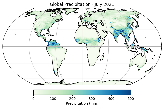
Visualize the results using CartoPy on an Equal Earth projection.

projection = ccrs.EqualEarth()
fig, ax = plt.subplots(1, 1, subplot_kw={'projection': projection})
fig.set_size_inches(10,5)

# Plot the data
plot = da_prcp.plot(
    ax=ax,
    transform=ccrs.PlateCarree(),  # Data is in PlateCarree
    cmap='GnBu',
    vmin=0, vmax=500,
    add_colorbar=False)

# Add a custom colorbar
cbar = fig.colorbar(plot, ax=ax, orientation='horizontal', shrink=0.5, pad=0.05)
cbar.set_label('Precipitation (mm)')
# Add coastlines and gridlines
ax.coastlines()
ax.gridlines()

# Set title
ax.set_title('Global Precipitation - July 2021')

# Show the plot
plt.show()

Finally save the results as a GeoTIFF file.

output_file = 'precipitation.tif'
output_path = os.path.join(output_folder, output_file)
da_prcp.rio.to_raster(output_path, compress='LZW')

---

If you want to give feedback or share your experience with this tutorial, please comment below. (requires GitHub account)