Calculating Climate Anomaly

Introduction

A climate anomaly refers to the difference between a measured climate variable and its long-term average or climatology. XArray provides many built-in methods to aggregate and compute statistical averages. In this tutorial, we explore these methods to calculate and visualize soil moisture anomalies.

Overview of the Task

We will take monthly gridded soil moisture data from NOAA Climate Prediction Center and calculate monthly anomalies relative to the 1971-2000 climatology.

Input Layers:

• soilw.mon.mean.v2.nc: A NetCDF file containing monthly mean soil moisture data from 1948 to current.

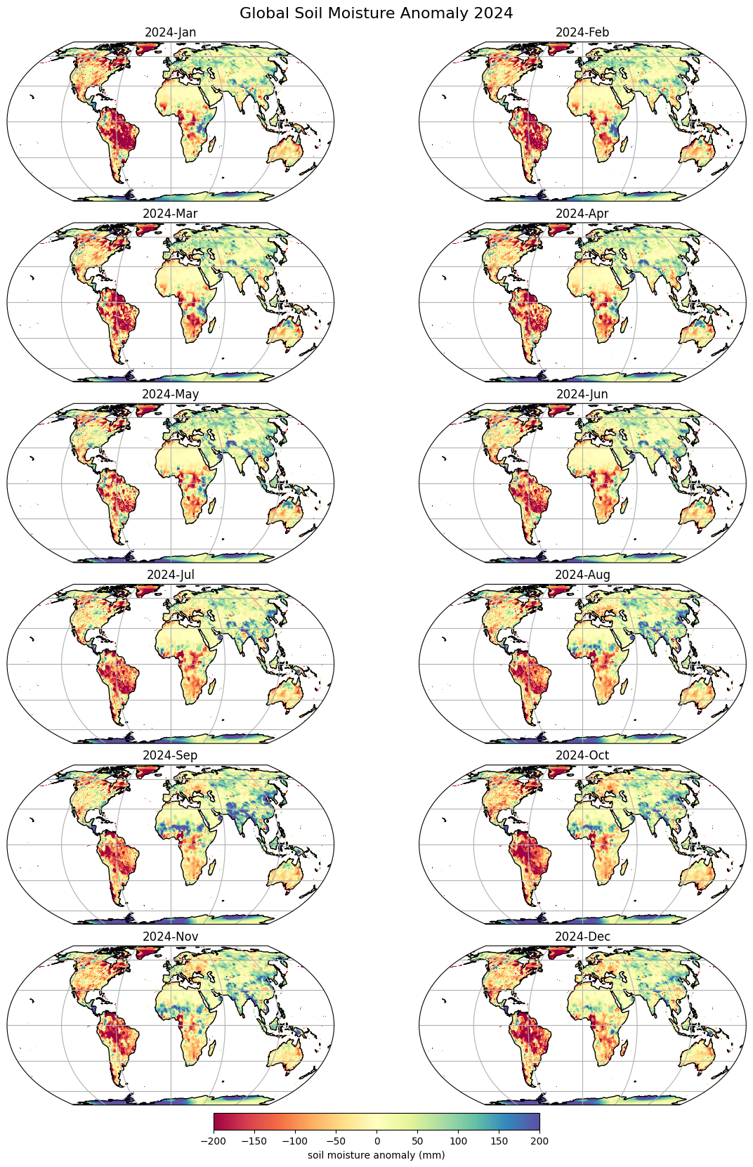
Output:

• Plots of monthly soil moisture anomalies for each month of 2024.

Data Credit:

• Global Soil Moisture. NOAA Climate Prediction Center. Retrieved 2025-02

Setup and Data Download

The following blocks of code will install the required packages and download the datasets to your Colab environment.

%%capture
if 'google.colab' in str(get_ipython()):
    !pip install cartopy

import cartopy
import cartopy.crs as ccrs
import matplotlib.pyplot as plt
import os
import pandas as pd
import xarray as xr

data_folder = 'data'
output_folder = 'output'

if not os.path.exists(data_folder):
    os.mkdir(data_folder)
if not os.path.exists(output_folder):
    os.mkdir(output_folder)

Data Pre-Processing

XArray can directly fetch data from a remote server. We specify the file path to the remote NetCDF file and open it.

filename = 'soilw.mon.mean.v2.nc'
server_url = 'https://psl.noaa.gov/thredds/fileServer/Datasets/cpcsoil/'
data_url = server_url + filename
ds = xr.open_dataset(data_url)
ds

<xarray.Dataset> Size: 959MB
Dimensions:  (lat: 360, lon: 720, time: 925)
Coordinates:
  * lat      (lat) float32 1kB 89.75 89.25 88.75 88.25 ... -88.75 -89.25 -89.75
  * lon      (lon) float32 3kB 0.25 0.75 1.25 1.75 ... 358.2 358.8 359.2 359.8
  * time     (time) datetime64[ns] 7kB 1948-01-01 1948-02-01 ... 2025-01-01
Data variables:
    soilw    (time, lat, lon) float32 959MB ...
Attributes:
    Conventions:    CF-1.0
    title:          CPC Soil Moisture
    institution:    NOAA/ESRL PSD
    dataset_title:  CPC Soil Moisture
    history:        Wed Oct 18 15:13:37 2017: ncks -d time,,-2 soilw.mon.mean...
    NCO:            4.6.9
    References:     https://www.psl.noaa.gov/data/gridded/data.cpcsoil.html
    source:         https://www.cpc.ncep.noaa.gov/products/Soilmst_Monitoring...

xarray.Dataset

• Dimensions:
  • lat: 360
  • lon: 720
  • time: 925
• Coordinates: (3)
  • lat
    (lat)
    float32
    89.75 89.25 88.75 ... -89.25 -89.75

    long_name :

    Latitude

    units :

    degrees_north

    actual_range :

    [ 89.75 -89.75]

    standard_name :

    latitude

    axis :

    Y

    coordinate_defines :

    point

    array([ 89.75,  89.25,  88.75, ..., -88.75, -89.25, -89.75], dtype=float32)

  • lon
    (lon)
    float32
    0.25 0.75 1.25 ... 359.2 359.8

    long_name :

    Longitude

    units :

    degrees_east

    actual_range :

    [2.5000e-01 3.5975e+02]

    standard_name :

    longitude

    axis :

    X

    coordinate_defines :

    point

    array([2.5000e-01, 7.5000e-01, 1.2500e+00, ..., 3.5875e+02, 3.5925e+02,
           3.5975e+02], dtype=float32)

  • time
    (time)
    datetime64[ns]
    1948-01-01 ... 2025-01-01

    long_name :

    Time

    delta_t :

    0000-01-00 00:00:00

    avg_period :

    0000-01-00 00:00:00

    standard_name :

    time

    axis :

    T

    bounds :

    time_bnds

    coordinate_defines :

    start

    prev_avg_period :

    0000-00-01 00:00:00

    actual_range :

    [54055. 82180.]

    array(['1948-01-01T00:00:00.000000000', '1948-02-01T00:00:00.000000000',
           '1948-03-01T00:00:00.000000000', ..., '2024-11-01T00:00:00.000000000',
           '2024-12-01T00:00:00.000000000', '2025-01-01T00:00:00.000000000'],
          dtype='datetime64[ns]')

• Data variables: (1)
  • soilw
    (time, lat, lon)
    float32
    ...

    long_name :

    Model-Calculated Monthly Mean Soil Moisture

    units :

    mm

    valid_range :

    [ 0. 1000.]

    dataset :

    CPC Monthly Soil Moisture

    var_desc :

    Soil Moisture

    level_desc :

    Surface

    statistic :

    Monthly Mean

    parent_stat :

    Other

    standard_name :

    lwe_thickness_of_soil_moisture_content

    cell_methods :

    time: mean (monthly from values)

    actual_range :

    [ 0. 756.0375]

    [239760000 values with dtype=float32]

• Indexes: (3)
  • lat
    PandasIndex

    PandasIndex(Index([ 89.75,  89.25,  88.75,  88.25,  87.75,  87.25,  86.75,  86.25,  85.75,
            85.25,
           ...
           -85.25, -85.75, -86.25, -86.75, -87.25, -87.75, -88.25, -88.75, -89.25,
           -89.75],
          dtype='float32', name='lat', length=360))

  • lon
    PandasIndex

    PandasIndex(Index([  0.25,   0.75,   1.25,   1.75,   2.25,   2.75,   3.25,   3.75,   4.25,
             4.75,
           ...
           355.25, 355.75, 356.25, 356.75, 357.25, 357.75, 358.25, 358.75, 359.25,
           359.75],
          dtype='float32', name='lon', length=720))

  • time
    PandasIndex

    PandasIndex(DatetimeIndex(['1948-01-01', '1948-02-01', '1948-03-01', '1948-04-01',
                   '1948-05-01', '1948-06-01', '1948-07-01', '1948-08-01',
                   '1948-09-01', '1948-10-01',
                   ...
                   '2024-04-01', '2024-05-01', '2024-06-01', '2024-07-01',
                   '2024-08-01', '2024-09-01', '2024-10-01', '2024-11-01',
                   '2024-12-01', '2025-01-01'],
                  dtype='datetime64[ns]', name='time', length=925, freq=None))

• Attributes: (8)

  Conventions :

  CF-1.0

  title :

  CPC Soil Moisture

  institution :

  NOAA/ESRL PSD

  dataset_title :

  CPC Soil Moisture

  history :

  Wed Oct 18 15:13:37 2017: ncks -d time,,-2 soilw.mon.mean.x.nc soilw.mon.mean.xx.nc Wed Oct 18 15:12:08 2017: ncks -d time,,-3 soilw.mon.mean.nc soilw.mon.mean.x.nc CPC Soil Moisture Obtained on Nov 2004 from CPC's website and written to netCDF by Cathy Smith 12/2004. he CPC Global monthly soil moisture dataset is a 1/2 degree resolution grid from 1948 to the present. The file is written in COARDS and CF compliant netCDF at NOAA ESRL/PSD https://www.esrl.noaa.gov/psd/ Converted to chunked, deflated non-packed NetCDF4 Jul 2014

  NCO :

  4.6.9

  References :

  https://www.psl.noaa.gov/data/gridded/data.cpcsoil.html

  source :

  https://www.cpc.ncep.noaa.gov/products/Soilmst_Monitoring/US/Soilmst/Soilmst.shtml

Select the soilw variable.

da = ds['soilw']
da

<xarray.DataArray 'soilw' (time: 925, lat: 360, lon: 720)> Size: 959MB
[239760000 values with dtype=float32]
Coordinates:
  * lat      (lat) float32 1kB 89.75 89.25 88.75 88.25 ... -88.75 -89.25 -89.75
  * lon      (lon) float32 3kB 0.25 0.75 1.25 1.75 ... 358.2 358.8 359.2 359.8
  * time     (time) datetime64[ns] 7kB 1948-01-01 1948-02-01 ... 2025-01-01
Attributes:
    long_name:      Model-Calculated Monthly Mean Soil Moisture
    units:          mm
    valid_range:    [   0. 1000.]
    dataset:        CPC Monthly Soil Moisture
    var_desc:       Soil Moisture
    level_desc:     Surface
    statistic:      Monthly Mean
    parent_stat:    Other
    standard_name:  lwe_thickness_of_soil_moisture_content
    cell_methods:   time: mean (monthly from values)
    actual_range:   [  0.     756.0375]

xarray.DataArray

'soilw'

• time: 925
• lat: 360
• lon: 720

• ...

  [239760000 values with dtype=float32]

• Coordinates: (3)
  • lat
    (lat)
    float32
    89.75 89.25 88.75 ... -89.25 -89.75

    long_name :

    Latitude

    units :

    degrees_north

    actual_range :

    [ 89.75 -89.75]

    standard_name :

    latitude

    axis :

    Y

    coordinate_defines :

    point

    array([ 89.75,  89.25,  88.75, ..., -88.75, -89.25, -89.75], dtype=float32)

  • lon
    (lon)
    float32
    0.25 0.75 1.25 ... 359.2 359.8

    long_name :

    Longitude

    units :

    degrees_east

    actual_range :

    [2.5000e-01 3.5975e+02]

    standard_name :

    longitude

    axis :

    X

    coordinate_defines :

    point

    array([2.5000e-01, 7.5000e-01, 1.2500e+00, ..., 3.5875e+02, 3.5925e+02,
           3.5975e+02], dtype=float32)

  • time
    (time)
    datetime64[ns]
    1948-01-01 ... 2025-01-01

    long_name :

    Time

    delta_t :

    0000-01-00 00:00:00

    avg_period :

    0000-01-00 00:00:00

    standard_name :

    time

    axis :

    T

    bounds :

    time_bnds

    coordinate_defines :

    start

    prev_avg_period :

    0000-00-01 00:00:00

    actual_range :

    [54055. 82180.]

    array(['1948-01-01T00:00:00.000000000', '1948-02-01T00:00:00.000000000',
           '1948-03-01T00:00:00.000000000', ..., '2024-11-01T00:00:00.000000000',
           '2024-12-01T00:00:00.000000000', '2025-01-01T00:00:00.000000000'],
          dtype='datetime64[ns]')

• Indexes: (3)
  • lat
    PandasIndex

    PandasIndex(Index([ 89.75,  89.25,  88.75,  88.25,  87.75,  87.25,  86.75,  86.25,  85.75,
            85.25,
           ...
           -85.25, -85.75, -86.25, -86.75, -87.25, -87.75, -88.25, -88.75, -89.25,
           -89.75],
          dtype='float32', name='lat', length=360))

  • lon
    PandasIndex

    PandasIndex(Index([  0.25,   0.75,   1.25,   1.75,   2.25,   2.75,   3.25,   3.75,   4.25,
             4.75,
           ...
           355.25, 355.75, 356.25, 356.75, 357.25, 357.75, 358.25, 358.75, 359.25,
           359.75],
          dtype='float32', name='lon', length=720))

  • time
    PandasIndex

    PandasIndex(DatetimeIndex(['1948-01-01', '1948-02-01', '1948-03-01', '1948-04-01',
                   '1948-05-01', '1948-06-01', '1948-07-01', '1948-08-01',
                   '1948-09-01', '1948-10-01',
                   ...
                   '2024-04-01', '2024-05-01', '2024-06-01', '2024-07-01',
                   '2024-08-01', '2024-09-01', '2024-10-01', '2024-11-01',
                   '2024-12-01', '2025-01-01'],
                  dtype='datetime64[ns]', name='time', length=925, freq=None))

• Attributes: (11)

  long_name :

  Model-Calculated Monthly Mean Soil Moisture

  units :

  mm

  valid_range :

  [ 0. 1000.]

  dataset :

  CPC Monthly Soil Moisture

  var_desc :

  Soil Moisture

  level_desc :

  Surface

  statistic :

  Monthly Mean

  parent_stat :

  Other

  standard_name :

  lwe_thickness_of_soil_moisture_content

  cell_methods :

  time: mean (monthly from values)

  actual_range :

  [ 0. 756.0375]

We transform the data from 0-360 longitude to -180 - +180 longitudes.

da.coords['lon'] = (da.coords['lon'] + 180) % 360 - 180
da = da.sortby(da.lon)

Calculating Anomaly

Let’s calculate soil moisture anomaly for 2021 as defined as the departure relative to the 1971–2000 climatology. We group the data by months and calculate monthly means across the entire time perid. We get a DataArray of 12 monthly means. Subtract the mean monthly soil moisture from each month to get the monthly anomalies.

%%time
mean = da.sel(time=slice('1971', '2000')).groupby('time.month').mean('time')
anomaly = da.groupby('time.month') - mean

We now plot the monthly anomaly for each month of 2024.

anomaly2024 = anomaly.sel(time='2024')

We create a layout with 12 subplots (6 rows and 2 columns). The result will be a 2D NumPy array of Axes for each subplot. To easily iterate over each, use use NumPy’s numpy.ndarray.flat attribute to get a flattened 1D array. The enumerate() function will give us the index of the array along with the Axes object from the array.

projection = ccrs.EqualEarth()

fig, axes = plt.subplots(6, 2, sharex=True, sharey=True,
                         constrained_layout=True,
                         subplot_kw={'projection': projection})
fig.set_size_inches(11.7, 16.5)


for index, ax in enumerate(axes.flat):
    data = anomaly2024.isel(time=index)
    im = data.plot(
        ax=ax,
        transform=ccrs.PlateCarree(),  # Data is in PlateCarree
        cmap='Spectral',
        vmin=-200, vmax=200,
        add_colorbar=False, add_labels=False)
    title = pd.to_datetime(data.time.values).strftime('%Y-%b')
    ax.set_title(title)
    ax.set_aspect('equal')
    # Add coastlines and gridlines
    ax.coastlines()
    ax.gridlines()

# Place the colorbar spanning the two bottom axes
fig.colorbar(im, ax=axes[5, :2], shrink=0.4, pad=0.05, location='bottom',
             label='soil moisture anomaly (mm)')
fig.suptitle('Global Soil Moisture Anomaly 2024', fontsize=16)
plt.show()

---

If you want to give feedback or share your experience with this tutorial, please comment below. (requires GitHub account)