Zonal Statistics with XArray

Introduction

Zonal Statistics analysis extracts a statistical summary of raster pixels within the zones of another dataset. The XArray ecosystem include rioxarray and xrspatial packages that can perform very fast statistical operations on geospatial rasters. We use these along with the geocube package to convert a vector layer to a rasterized XArray dataset. This approach ensures you leverage the efficiences of XArray and result in performance that is magnitudes faster than other approaches (i.e. with rasterstats).

Overview of the Task

We will use a gridded precipitation raster and extract the mean total precipitaion for each county in the state of California, USA.

Input Layers:

• chirps-v2.0.2021.tif: Raster grid of precipitaion for 2021 by Climate Hazards Group InfraRed Precipitation with Station data (CHIRPS) for 2021.

• cb_2021_us_county_500k.zip: A vector file with polygons representing counties in the US.

Output Layers:

• precipitation.gpkg : A GeoPackage containing a vector layer of county polygon with total precipitaion values sampled from the raster.

Data Credit:

• CHIRPS 2021 precipitation. Climate Hazards Center (CHC). Retrieved 2022-09

• US Census files: 2021 United States Census Bureau. Retrieved 2022-09.

Setup and Data Download

The following blocks of code will install the required packages and download the datasets to your Colab environment.

%%capture
if 'google.colab' in str(get_ipython()):
    !pip install rioxarray geocube xarray_spatial

import os
import pandas as pd
import geopandas as gpd
import rioxarray as rxr
import matplotlib.pyplot as plt
from geocube.api.core import make_geocube
from xrspatial import zonal_stats

data_folder = 'data'
output_folder = 'output'

if not os.path.exists(data_folder):
    os.mkdir(data_folder)
if not os.path.exists(output_folder):
    os.mkdir(output_folder)

def download(url):
    filename = os.path.join(data_folder, os.path.basename(url))
    if not os.path.exists(filename):
        from urllib.request import urlretrieve
        local, _ = urlretrieve(url, filename)
        print('Downloaded ' + local)

raster_file = 'chirps-v2.0.2021.tif'
zones_file = 'cb_2021_us_county_500k.zip'

files = [
    'https://data.chc.ucsb.edu/products/CHIRPS-2.0/global_annual/tifs/' + raster_file,
    'https://www2.census.gov/geo/tiger/GENZ2021/shp/' + zones_file,
]

for file in files:
  download(file)

Data Pre-Processing

First we will read the Zipped counties shapefile and filter out the counties that are in California state.

The dataframe has a column as STATE_NAME having naesm of states that can be used to filter the counties for California.

zones_file_path = os.path.join(data_folder, zones_file)

zones_df = gpd.read_file(zones_file_path)
california_df  = zones_df[zones_df['STATE_NAME'] == 'California'].copy()
california_df.iloc[:5, :5]

	STATEFP	COUNTYFP	COUNTYNS	AFFGEOID	GEOID
47	06	059	00277294	0500000US06059	06059
50	06	111	00277320	0500000US06111	06111
94	06	063	00277296	0500000US06063	06063
181	06	015	01682074	0500000US06015	06015
245	06	023	01681908	0500000US06023	06023

The ‘GEOID’ column contains a unique id for all the counties present in the state, but it is of object type. We need to convert it to int type to be used in xarray.

Since the CHIRPS dataset is for whole world, so we clip it to the bounds of California state. Storing the values of bounding box in the required variables.

Now, read the raster file using rioxarray and clip it to the geometry of California state.

raster_filepath = os.path.join(data_folder, raster_file)
raster = rxr.open_rasterio(raster_filepath, mask_and_scale=True)
clipped = raster.rio.clip(california_df.geometry)
clipped

<xarray.DataArray (band: 1, y: 189, x: 205)> Size: 155kB
array([[[nan, nan, nan, ..., nan, nan, nan],
        [nan, nan, nan, ..., nan, nan, nan],
        [nan, nan, nan, ..., nan, nan, nan],
        ...,
        [nan, nan, nan, ..., nan, nan, nan],
        [nan, nan, nan, ..., nan, nan, nan],
        [nan, nan, nan, ..., nan, nan, nan]]], dtype=float32)
Coordinates:
  * band         (band) int64 8B 1
  * x            (x) float64 2kB -124.4 -124.3 -124.3 ... -114.3 -114.2 -114.2
  * y            (y) float64 2kB 41.97 41.92 41.87 41.82 ... 32.67 32.62 32.57
    spatial_ref  int64 8B 0
Attributes:
    TIFFTAG_DOCUMENTNAME:      /home/CHIRPS/annual/v2.0/chirps-v2.0.2021.tif
    TIFFTAG_IMAGEDESCRIPTION:  IDL TIFF file
    TIFFTAG_SOFTWARE:          IDL 8.7.2, Harris Geospatial Solutions, Inc.
    TIFFTAG_DATETIME:          2022:01:18 14:24:32
    TIFFTAG_XRESOLUTION:       100
    TIFFTAG_YRESOLUTION:       100
    TIFFTAG_RESOLUTIONUNIT:    2 (pixels/inch)
    AREA_OR_POINT:             Area

xarray.DataArray

• band: 1
• y: 189
• x: 205

• nan nan nan nan 971.1 2.659e+03 2.618e+03 ... nan nan nan nan nan nan

  array([[[nan, nan, nan, ..., nan, nan, nan],
          [nan, nan, nan, ..., nan, nan, nan],
          [nan, nan, nan, ..., nan, nan, nan],
          ...,
          [nan, nan, nan, ..., nan, nan, nan],
          [nan, nan, nan, ..., nan, nan, nan],
          [nan, nan, nan, ..., nan, nan, nan]]], dtype=float32)

• Coordinates: (4)
  • band
    (band)
    int64
    1

    array([1])

  • x
    (x)
    float64
    -124.4 -124.3 ... -114.2 -114.2

    axis :

    X

    long_name :

    longitude

    standard_name :

    longitude

    units :

    degrees_east

    array([-124.374999, -124.324999, -124.274999, ..., -114.274999, -114.224999,
           -114.174999])

  • y
    (y)
    float64
    41.97 41.92 41.87 ... 32.62 32.57

    axis :

    Y

    long_name :

    latitude

    standard_name :

    latitude

    units :

    degrees_north

    array([41.975, 41.925, 41.875, 41.825, 41.775, 41.725, 41.675, 41.625, 41.575,
           41.525, 41.475, 41.425, 41.375, 41.325, 41.275, 41.225, 41.175, 41.125,
           41.075, 41.025, 40.975, 40.925, 40.875, 40.825, 40.775, 40.725, 40.675,
           40.625, 40.575, 40.525, 40.475, 40.425, 40.375, 40.325, 40.275, 40.225,
           40.175, 40.125, 40.075, 40.025, 39.975, 39.925, 39.875, 39.825, 39.775,
           39.725, 39.675, 39.625, 39.575, 39.525, 39.475, 39.425, 39.375, 39.325,
           39.275, 39.225, 39.175, 39.125, 39.075, 39.025, 38.975, 38.925, 38.875,
           38.825, 38.775, 38.725, 38.675, 38.625, 38.575, 38.525, 38.475, 38.425,
           38.375, 38.325, 38.275, 38.225, 38.175, 38.125, 38.075, 38.025, 37.975,
           37.925, 37.875, 37.825, 37.775, 37.725, 37.675, 37.625, 37.575, 37.525,
           37.475, 37.425, 37.375, 37.325, 37.275, 37.225, 37.175, 37.125, 37.075,
           37.025, 36.975, 36.925, 36.875, 36.825, 36.775, 36.725, 36.675, 36.625,
           36.575, 36.525, 36.475, 36.425, 36.375, 36.325, 36.275, 36.225, 36.175,
           36.125, 36.075, 36.025, 35.975, 35.925, 35.875, 35.825, 35.775, 35.725,
           35.675, 35.625, 35.575, 35.525, 35.475, 35.425, 35.375, 35.325, 35.275,
           35.225, 35.175, 35.125, 35.075, 35.025, 34.975, 34.925, 34.875, 34.825,
           34.775, 34.725, 34.675, 34.625, 34.575, 34.525, 34.475, 34.425, 34.375,
           34.325, 34.275, 34.225, 34.175, 34.125, 34.075, 34.025, 33.975, 33.925,
           33.875, 33.825, 33.775, 33.725, 33.675, 33.625, 33.575, 33.525, 33.475,
           33.425, 33.375, 33.325, 33.275, 33.225, 33.175, 33.125, 33.075, 33.025,
           32.975, 32.925, 32.875, 32.825, 32.775, 32.725, 32.675, 32.625, 32.575])

  • spatial_ref
    ()
    int64
    0

    crs_wkt :

    GEOGCS["WGS 84",DATUM["WGS_1984",SPHEROID["WGS 84",6378137,298.257223563,AUTHORITY["EPSG","7030"]],AUTHORITY["EPSG","6326"]],PRIMEM["Greenwich",0,AUTHORITY["EPSG","8901"]],UNIT["degree",0.0174532925199433,AUTHORITY["EPSG","9122"]],AXIS["Latitude",NORTH],AXIS["Longitude",EAST],AUTHORITY["EPSG","4326"]]

    semi_major_axis :

    6378137.0

    semi_minor_axis :

    6356752.314245179

    inverse_flattening :

    298.257223563

    reference_ellipsoid_name :

    WGS 84

    longitude_of_prime_meridian :

    0.0

    prime_meridian_name :

    Greenwich

    geographic_crs_name :

    WGS 84

    horizontal_datum_name :

    World Geodetic System 1984

    grid_mapping_name :

    latitude_longitude

    spatial_ref :

    GEOGCS["WGS 84",DATUM["WGS_1984",SPHEROID["WGS 84",6378137,298.257223563,AUTHORITY["EPSG","7030"]],AUTHORITY["EPSG","6326"]],PRIMEM["Greenwich",0,AUTHORITY["EPSG","8901"]],UNIT["degree",0.0174532925199433,AUTHORITY["EPSG","9122"]],AXIS["Latitude",NORTH],AXIS["Longitude",EAST],AUTHORITY["EPSG","4326"]]

    GeoTransform :

    -124.39999917149544 0.05000000074505806 0.0 41.99999988079071 0.0 -0.05000000074505806

    array(0)

• Indexes: (3)
  • band
    PandasIndex

    PandasIndex(Index([1], dtype='int64', name='band'))

  • x
    PandasIndex

    PandasIndex(Index([-124.37499917112291, -124.32499917037785, -124.27499916963279,
           -124.22499916888773, -124.17499916814268, -124.12499916739762,
           -124.07499916665256,  -124.0249991659075, -123.97499916516244,
           -123.92499916441739,
           ...
           -114.62499902583659, -114.57499902509153, -114.52499902434647,
           -114.47499902360141, -114.42499902285635,  -114.3749990221113,
           -114.32499902136624, -114.27499902062118, -114.22499901987612,
           -114.17499901913106],
          dtype='float64', name='x', length=205))

  • y
    PandasIndex

    PandasIndex(Index([ 41.97499988041818,  41.92499987967312, 41.874999878928065,
            41.82499987818301,  41.77499987743795,  41.72499987669289,
            41.67499987594783, 41.624999875202775,  41.57499987445772,
            41.52499987371266,
           ...
            33.02499974705279,  32.97499974630773,  32.92499974556267,
           32.874999744817615,  32.82499974407256,   32.7749997433275,
            32.72499974258244,  32.67499974183738, 32.624999741092324,
           32.574999740347266],
          dtype='float64', name='y', length=189))

• Attributes: (8)

  TIFFTAG_DOCUMENTNAME :

  /home/CHIRPS/annual/v2.0/chirps-v2.0.2021.tif

  TIFFTAG_IMAGEDESCRIPTION :

  IDL TIFF file

  TIFFTAG_SOFTWARE :

  IDL 8.7.2, Harris Geospatial Solutions, Inc.

  TIFFTAG_DATETIME :

  2022:01:18 14:24:32

  TIFFTAG_XRESOLUTION :

  100

  TIFFTAG_YRESOLUTION :

  100

  TIFFTAG_RESOLUTIONUNIT :

  2 (pixels/inch)

  AREA_OR_POINT :

  Area

You will notice that the raster has many pixels with value -9999. These are NoData values but they are not encoded as such. We will mask these values to get only the valid pixels.

The raster has only 1 band containing yearly precipitaion values, so we select it.

precipitation = clipped.sel(band=1)
precipitation

<xarray.DataArray (y: 189, x: 205)> Size: 155kB
array([[nan, nan, nan, ..., nan, nan, nan],
       [nan, nan, nan, ..., nan, nan, nan],
       [nan, nan, nan, ..., nan, nan, nan],
       ...,
       [nan, nan, nan, ..., nan, nan, nan],
       [nan, nan, nan, ..., nan, nan, nan],
       [nan, nan, nan, ..., nan, nan, nan]], dtype=float32)
Coordinates:
    band         int64 8B 1
  * x            (x) float64 2kB -124.4 -124.3 -124.3 ... -114.3 -114.2 -114.2
  * y            (y) float64 2kB 41.97 41.92 41.87 41.82 ... 32.67 32.62 32.57
    spatial_ref  int64 8B 0
Attributes:
    TIFFTAG_DOCUMENTNAME:      /home/CHIRPS/annual/v2.0/chirps-v2.0.2021.tif
    TIFFTAG_IMAGEDESCRIPTION:  IDL TIFF file
    TIFFTAG_SOFTWARE:          IDL 8.7.2, Harris Geospatial Solutions, Inc.
    TIFFTAG_DATETIME:          2022:01:18 14:24:32
    TIFFTAG_XRESOLUTION:       100
    TIFFTAG_YRESOLUTION:       100
    TIFFTAG_RESOLUTIONUNIT:    2 (pixels/inch)
    AREA_OR_POINT:             Area

xarray.DataArray

• y: 189
• x: 205

• nan nan nan nan 971.1 2.659e+03 2.618e+03 ... nan nan nan nan nan nan

  array([[nan, nan, nan, ..., nan, nan, nan],
         [nan, nan, nan, ..., nan, nan, nan],
         [nan, nan, nan, ..., nan, nan, nan],
         ...,
         [nan, nan, nan, ..., nan, nan, nan],
         [nan, nan, nan, ..., nan, nan, nan],
         [nan, nan, nan, ..., nan, nan, nan]], dtype=float32)

• Coordinates: (4)
  • band
    ()
    int64
    1

    array(1)

  • x
    (x)
    float64
    -124.4 -124.3 ... -114.2 -114.2

    axis :

    X

    long_name :

    longitude

    standard_name :

    longitude

    units :

    degrees_east

    array([-124.374999, -124.324999, -124.274999, ..., -114.274999, -114.224999,
           -114.174999])

  • y
    (y)
    float64
    41.97 41.92 41.87 ... 32.62 32.57

    axis :

    Y

    long_name :

    latitude

    standard_name :

    latitude

    units :

    degrees_north

    array([41.975, 41.925, 41.875, 41.825, 41.775, 41.725, 41.675, 41.625, 41.575,
           41.525, 41.475, 41.425, 41.375, 41.325, 41.275, 41.225, 41.175, 41.125,
           41.075, 41.025, 40.975, 40.925, 40.875, 40.825, 40.775, 40.725, 40.675,
           40.625, 40.575, 40.525, 40.475, 40.425, 40.375, 40.325, 40.275, 40.225,
           40.175, 40.125, 40.075, 40.025, 39.975, 39.925, 39.875, 39.825, 39.775,
           39.725, 39.675, 39.625, 39.575, 39.525, 39.475, 39.425, 39.375, 39.325,
           39.275, 39.225, 39.175, 39.125, 39.075, 39.025, 38.975, 38.925, 38.875,
           38.825, 38.775, 38.725, 38.675, 38.625, 38.575, 38.525, 38.475, 38.425,
           38.375, 38.325, 38.275, 38.225, 38.175, 38.125, 38.075, 38.025, 37.975,
           37.925, 37.875, 37.825, 37.775, 37.725, 37.675, 37.625, 37.575, 37.525,
           37.475, 37.425, 37.375, 37.325, 37.275, 37.225, 37.175, 37.125, 37.075,
           37.025, 36.975, 36.925, 36.875, 36.825, 36.775, 36.725, 36.675, 36.625,
           36.575, 36.525, 36.475, 36.425, 36.375, 36.325, 36.275, 36.225, 36.175,
           36.125, 36.075, 36.025, 35.975, 35.925, 35.875, 35.825, 35.775, 35.725,
           35.675, 35.625, 35.575, 35.525, 35.475, 35.425, 35.375, 35.325, 35.275,
           35.225, 35.175, 35.125, 35.075, 35.025, 34.975, 34.925, 34.875, 34.825,
           34.775, 34.725, 34.675, 34.625, 34.575, 34.525, 34.475, 34.425, 34.375,
           34.325, 34.275, 34.225, 34.175, 34.125, 34.075, 34.025, 33.975, 33.925,
           33.875, 33.825, 33.775, 33.725, 33.675, 33.625, 33.575, 33.525, 33.475,
           33.425, 33.375, 33.325, 33.275, 33.225, 33.175, 33.125, 33.075, 33.025,
           32.975, 32.925, 32.875, 32.825, 32.775, 32.725, 32.675, 32.625, 32.575])

  • spatial_ref
    ()
    int64
    0

    crs_wkt :

    GEOGCS["WGS 84",DATUM["WGS_1984",SPHEROID["WGS 84",6378137,298.257223563,AUTHORITY["EPSG","7030"]],AUTHORITY["EPSG","6326"]],PRIMEM["Greenwich",0,AUTHORITY["EPSG","8901"]],UNIT["degree",0.0174532925199433,AUTHORITY["EPSG","9122"]],AXIS["Latitude",NORTH],AXIS["Longitude",EAST],AUTHORITY["EPSG","4326"]]

    semi_major_axis :

    6378137.0

    semi_minor_axis :

    6356752.314245179

    inverse_flattening :

    298.257223563

    reference_ellipsoid_name :

    WGS 84

    longitude_of_prime_meridian :

    0.0

    prime_meridian_name :

    Greenwich

    geographic_crs_name :

    WGS 84

    horizontal_datum_name :

    World Geodetic System 1984

    grid_mapping_name :

    latitude_longitude

    spatial_ref :

    GEOGCS["WGS 84",DATUM["WGS_1984",SPHEROID["WGS 84",6378137,298.257223563,AUTHORITY["EPSG","7030"]],AUTHORITY["EPSG","6326"]],PRIMEM["Greenwich",0,AUTHORITY["EPSG","8901"]],UNIT["degree",0.0174532925199433,AUTHORITY["EPSG","9122"]],AXIS["Latitude",NORTH],AXIS["Longitude",EAST],AUTHORITY["EPSG","4326"]]

    GeoTransform :

    -124.39999917149544 0.05000000074505806 0.0 41.99999988079071 0.0 -0.05000000074505806

    array(0)

• Indexes: (2)
  • x
    PandasIndex

    PandasIndex(Index([-124.37499917112291, -124.32499917037785, -124.27499916963279,
           -124.22499916888773, -124.17499916814268, -124.12499916739762,
           -124.07499916665256,  -124.0249991659075, -123.97499916516244,
           -123.92499916441739,
           ...
           -114.62499902583659, -114.57499902509153, -114.52499902434647,
           -114.47499902360141, -114.42499902285635,  -114.3749990221113,
           -114.32499902136624, -114.27499902062118, -114.22499901987612,
           -114.17499901913106],
          dtype='float64', name='x', length=205))

  • y
    PandasIndex

    PandasIndex(Index([ 41.97499988041818,  41.92499987967312, 41.874999878928065,
            41.82499987818301,  41.77499987743795,  41.72499987669289,
            41.67499987594783, 41.624999875202775,  41.57499987445772,
            41.52499987371266,
           ...
            33.02499974705279,  32.97499974630773,  32.92499974556267,
           32.874999744817615,  32.82499974407256,   32.7749997433275,
            32.72499974258244,  32.67499974183738, 32.624999741092324,
           32.574999740347266],
          dtype='float64', name='y', length=189))

• Attributes: (8)

  TIFFTAG_DOCUMENTNAME :

  /home/CHIRPS/annual/v2.0/chirps-v2.0.2021.tif

  TIFFTAG_IMAGEDESCRIPTION :

  IDL TIFF file

  TIFFTAG_SOFTWARE :

  IDL 8.7.2, Harris Geospatial Solutions, Inc.

  TIFFTAG_DATETIME :

  2022:01:18 14:24:32

  TIFFTAG_XRESOLUTION :

  100

  TIFFTAG_YRESOLUTION :

  100

  TIFFTAG_RESOLUTIONUNIT :

  2 (pixels/inch)

  AREA_OR_POINT :

  Area

Sampling Raster Values

Now we will extract the value of the raster pixels for every counties in California. We will be using the geocube module for that. It takes geodataframe, it’s unique value as integer and a xarray dataset as input and converts the geodataframe into a xarray dataset having dimension and coordinates same as of given input xarray dataset

california_df['GEOID'] = california_df.GEOID.astype(int)
california_raster = make_geocube(
    vector_data=california_df,
    measurements=['GEOID'],
    like=precipitation,
)
california_raster

<xarray.Dataset> Size: 313kB
Dimensions:      (y: 189, x: 205)
Coordinates:
  * y            (y) float64 2kB 41.97 41.92 41.87 41.82 ... 32.67 32.62 32.57
  * x            (x) float64 2kB -124.4 -124.3 -124.3 ... -114.3 -114.2 -114.2
    spatial_ref  int64 8B 0
Data variables:
    GEOID        (y, x) float64 310kB nan nan nan nan ... nan nan nan nan

xarray.Dataset

• Dimensions:
  • y: 189
  • x: 205
• Coordinates: (3)
  • y
    (y)
    float64
    41.97 41.92 41.87 ... 32.62 32.57

    axis :

    Y

    long_name :

    latitude

    standard_name :

    latitude

    units :

    degrees_north

    array([41.975, 41.925, 41.875, 41.825, 41.775, 41.725, 41.675, 41.625, 41.575,
           41.525, 41.475, 41.425, 41.375, 41.325, 41.275, 41.225, 41.175, 41.125,
           41.075, 41.025, 40.975, 40.925, 40.875, 40.825, 40.775, 40.725, 40.675,
           40.625, 40.575, 40.525, 40.475, 40.425, 40.375, 40.325, 40.275, 40.225,
           40.175, 40.125, 40.075, 40.025, 39.975, 39.925, 39.875, 39.825, 39.775,
           39.725, 39.675, 39.625, 39.575, 39.525, 39.475, 39.425, 39.375, 39.325,
           39.275, 39.225, 39.175, 39.125, 39.075, 39.025, 38.975, 38.925, 38.875,
           38.825, 38.775, 38.725, 38.675, 38.625, 38.575, 38.525, 38.475, 38.425,
           38.375, 38.325, 38.275, 38.225, 38.175, 38.125, 38.075, 38.025, 37.975,
           37.925, 37.875, 37.825, 37.775, 37.725, 37.675, 37.625, 37.575, 37.525,
           37.475, 37.425, 37.375, 37.325, 37.275, 37.225, 37.175, 37.125, 37.075,
           37.025, 36.975, 36.925, 36.875, 36.825, 36.775, 36.725, 36.675, 36.625,
           36.575, 36.525, 36.475, 36.425, 36.375, 36.325, 36.275, 36.225, 36.175,
           36.125, 36.075, 36.025, 35.975, 35.925, 35.875, 35.825, 35.775, 35.725,
           35.675, 35.625, 35.575, 35.525, 35.475, 35.425, 35.375, 35.325, 35.275,
           35.225, 35.175, 35.125, 35.075, 35.025, 34.975, 34.925, 34.875, 34.825,
           34.775, 34.725, 34.675, 34.625, 34.575, 34.525, 34.475, 34.425, 34.375,
           34.325, 34.275, 34.225, 34.175, 34.125, 34.075, 34.025, 33.975, 33.925,
           33.875, 33.825, 33.775, 33.725, 33.675, 33.625, 33.575, 33.525, 33.475,
           33.425, 33.375, 33.325, 33.275, 33.225, 33.175, 33.125, 33.075, 33.025,
           32.975, 32.925, 32.875, 32.825, 32.775, 32.725, 32.675, 32.625, 32.575])

  • x
    (x)
    float64
    -124.4 -124.3 ... -114.2 -114.2

    axis :

    X

    long_name :

    longitude

    standard_name :

    longitude

    units :

    degrees_east

    array([-124.374999, -124.324999, -124.274999, ..., -114.274999, -114.224999,
           -114.174999])

  • spatial_ref
    ()
    int64
    0

    crs_wkt :

    GEOGCS["WGS 84",DATUM["WGS_1984",SPHEROID["WGS 84",6378137,298.257223563,AUTHORITY["EPSG","7030"]],AUTHORITY["EPSG","6326"]],PRIMEM["Greenwich",0,AUTHORITY["EPSG","8901"]],UNIT["degree",0.0174532925199433,AUTHORITY["EPSG","9122"]],AXIS["Latitude",NORTH],AXIS["Longitude",EAST],AUTHORITY["EPSG","4326"]]

    semi_major_axis :

    6378137.0

    semi_minor_axis :

    6356752.314245179

    inverse_flattening :

    298.257223563

    reference_ellipsoid_name :

    WGS 84

    longitude_of_prime_meridian :

    0.0

    prime_meridian_name :

    Greenwich

    geographic_crs_name :

    WGS 84

    horizontal_datum_name :

    World Geodetic System 1984

    grid_mapping_name :

    latitude_longitude

    spatial_ref :

    GEOGCS["WGS 84",DATUM["WGS_1984",SPHEROID["WGS 84",6378137,298.257223563,AUTHORITY["EPSG","7030"]],AUTHORITY["EPSG","6326"]],PRIMEM["Greenwich",0,AUTHORITY["EPSG","8901"]],UNIT["degree",0.0174532925199433,AUTHORITY["EPSG","9122"]],AXIS["Latitude",NORTH],AXIS["Longitude",EAST],AUTHORITY["EPSG","4326"]]

    GeoTransform :

    -124.39999917149544 0.05000000074505806 0.0 41.99999988079071 0.0 -0.05000000074505806

    array(0)

• Data variables: (1)
  • GEOID
    (y, x)
    float64
    nan nan nan nan ... nan nan nan nan

    name :

    GEOID

    long_name :

    GEOID

    _FillValue :

    nan

    array([[nan, nan, nan, ..., nan, nan, nan],
           [nan, nan, nan, ..., nan, nan, nan],
           [nan, nan, nan, ..., nan, nan, nan],
           ...,
           [nan, nan, nan, ..., nan, nan, nan],
           [nan, nan, nan, ..., nan, nan, nan],
           [nan, nan, nan, ..., nan, nan, nan]])

• Indexes: (2)
  • y
    PandasIndex

    PandasIndex(Index([ 41.97499988041818,  41.92499987967312, 41.874999878928065,
            41.82499987818301,  41.77499987743795,  41.72499987669289,
            41.67499987594783, 41.624999875202775,  41.57499987445772,
            41.52499987371266,
           ...
            33.02499974705279,  32.97499974630773,  32.92499974556267,
           32.874999744817615,  32.82499974407256,   32.7749997433275,
            32.72499974258244,  32.67499974183738, 32.624999741092324,
           32.574999740347266],
          dtype='float64', name='y', length=189))

  • x
    PandasIndex

    PandasIndex(Index([-124.37499917112291, -124.32499917037785, -124.27499916963279,
           -124.22499916888773, -124.17499916814268, -124.12499916739762,
           -124.07499916665256,  -124.0249991659075, -123.97499916516244,
           -123.92499916441739,
           ...
           -114.62499902583659, -114.57499902509153, -114.52499902434647,
           -114.47499902360141, -114.42499902285635,  -114.3749990221113,
           -114.32499902136624, -114.27499902062118, -114.22499901987612,
           -114.17499901913106],
          dtype='float64', name='x', length=205))

• Attributes: (0)

Now we can use the Zonal Stats function from xarray-spatial to compute various statistics for each zone.

stats_df = zonal_stats(zones=california_raster.GEOID, values=precipitation)
stats_df.iloc[:5]

	zone	mean	max	min	sum	std	var	count
0	6001.0	371.543365	607.836914	177.121490	29351.925781	90.103966	8118.724121	79.0
1	6003.0	709.821960	1099.949951	481.242493	56075.933594	130.407578	17006.134766	79.0
2	6005.0	748.022400	1076.544678	416.273926	50117.500000	202.018219	40811.359375	67.0
3	6007.0	720.174438	1303.399902	428.850677	135392.796875	233.186996	54376.171875	188.0
4	6009.0	680.377014	1204.727417	314.935669	74161.093750	233.036972	54306.230469	109.0

We select the required statistics and join the results with the original layer.

stats_df['GEOID'] = stats_df['zone'].astype(int)
joined = california_df.merge(stats_df[['GEOID', 'mean']], on='GEOID')
joined.iloc[:5, -5:]

	LSAD	ALAND	AWATER	geometry	mean
0	06	2053476505	406279630	POLYGON ((-118.11442 33.74518, -118.11305 33.7...	262.130493
1	06	4767622161	947345735	MULTIPOLYGON (((-119.44123 34.01408, -119.4366...	339.915070
2	06	6612400772	156387638	POLYGON ((-121.49703 40.43702, -121.49487 40.4...	834.308716
3	06	2606118035	578742633	MULTIPOLYGON (((-124.2175 41.95081, -124.21704...	2439.237549
4	06	9241565229	1253726036	POLYGON ((-124.4086 40.4432, -124.39664 40.462...	1273.892456

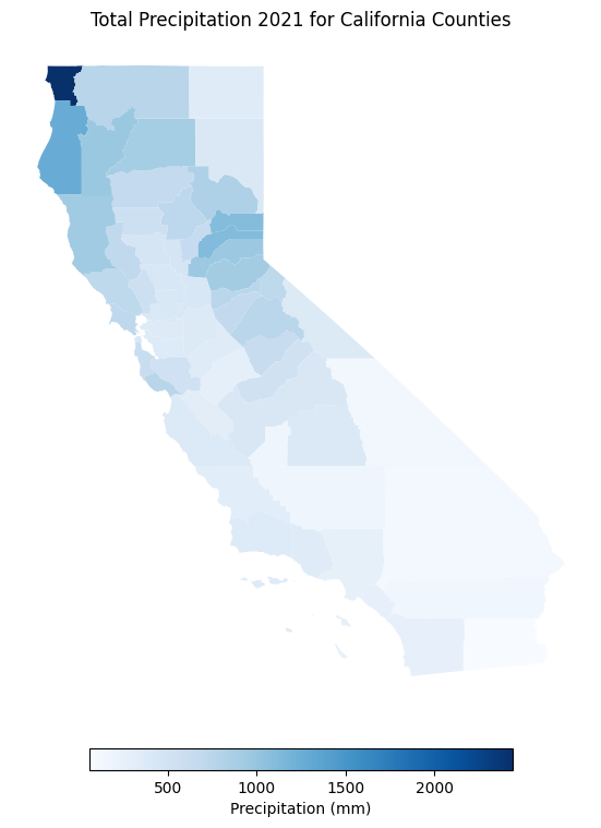
Let’s plot and visualize the results. The map shows the average annual precipitation for each county in California.

fig, ax = plt.subplots(1, 1)
fig.set_size_inches(10,10)

legend_kwds={
           'orientation': 'horizontal',  # Make the legend horizontal
           'shrink': 0.5,  # Reduce the size of the legend bar by 50%
           'pad': 0.05,  # Add some padding around the legend
           'label': 'Precipitation (mm)',  # Set the legend label (optional)
       }
joined.plot(ax=ax, column='mean', cmap='Blues',
          legend=True, legend_kwds=legend_kwds)
ax.set_axis_off()
ax.set_title('Total Precipitation 2021 for California Counties')
plt.show()

Finally, we save the sampled result to disk as .gpkg.

output_file = 'precipitation_by_county.gpkg'
output_path = os.path.join(output_folder, output_file)

joined.to_file(driver = 'GPKG', filename =output_path)
print('Successfully written output file at {}'.format(output_path))

Successfully written output file at output/precipitation_by_county.gpkg

---

If you want to give feedback or share your experience with this tutorial, please comment below. (requires GitHub account)