Basic Raster Styling and Analysis

Introduction

rioxarray and xarray-spatial extensions provide core functionality for working with geospatial rasters using XArray. In this tutorial, we will use these to read, analyze and reclassify population rasters.

Overview of the Task

We will use the Gridded Population of the World (GPW) v4 dataset from Columbia University. Specifically, the Population Count for the entire globe at 2.5 Minute (~5Km) resolution in GeoTiFF format and for the year 2010 and 2020. Using these we will create a thematic map of the global population change between year 2010 and 2020.

Input Layers:

• gpw-v4-population-count-rev11_YYYY_2pt5_min_tif.zip: Zipped Raster files having population data.

Output:

• change_class.tif : A GeoTIFF file of categorized population change.

Data Credit:

• Center for International Earth Science Information Network - CIESIN - Columbia University. 2018. Gridded Population of the World, Version 4 (GPWv4): Population Count, Revision 11. Palisades, NY: NASA Socioeconomic Data and Applications Center (SEDAC). https://doi.org/10.7927/H4JW8BX5. Accessed 27 JUNE 2019

Watch Video Walkthrough

Setup and Data Download

The following blocks of code will install the required packages and download the datasets to your Colab environment.

%%capture
if 'google.colab' in str(get_ipython()):
    !pip install rioxarray xarray-spatial

import numpy as np
import matplotlib.pyplot as plt
import matplotlib.patches as mpatches
import os
import rioxarray as rxr
import xrspatial
import zipfile

data_folder = 'data'
output_folder = 'output'

if not os.path.exists(data_folder):
    os.mkdir(data_folder)
if not os.path.exists(output_folder):
    os.mkdir(output_folder)

def download(url):
    filename = os.path.join(data_folder, os.path.basename(url))
    if not os.path.exists(filename):
        from urllib.request import urlretrieve
        local, _ = urlretrieve(url, filename)
        print('Downloaded ' + local)

data_url = 'https://github.com/spatialthoughts/geopython-tutorials/releases/download/data/'

gpw_pop_2010 = 'gpw-v4-population-count-rev11_2010_2pt5_min_tif.zip'
gpw_pop_2020 = 'gpw-v4-population-count-rev11_2020_2pt5_min_tif.zip'

download(data_url + gpw_pop_2010)
download(data_url + gpw_pop_2020)

Downloaded data/gpw-v4-population-count-rev11_2010_2pt5_min_tif.zip
Downloaded data/gpw-v4-population-count-rev11_2020_2pt5_min_tif.zip

Procedure

Read the gridded population of the World files using the rioxarray by using open_raster function. We can read the GeoTIFF file directly from the zip archive without uncompressing it first by creating a URI with the zip:// prefix.

gpw_pop_2010_path = os.path.join(data_folder, gpw_pop_2010)

with zipfile.ZipFile(gpw_pop_2010_path) as f:
  files = f.namelist()
  for file in files:
    if os.path.splitext(file)[1] == '.tif':
      tif_file = file

gpw_pop_2010_uri = 'zip://{}!{}'.format(gpw_pop_2010_path, tif_file)
pop2010 = rxr.open_rasterio(gpw_pop_2010_uri, mask_and_scale=True)

gpw_pop_2020_path = os.path.join(data_folder, gpw_pop_2020)

with zipfile.ZipFile(gpw_pop_2020_path) as f:
  files = f.namelist()
  for file in files:
    if os.path.splitext(file)[1] == '.tif':
      tif_file = file

gpw_pop_2020_uri = 'zip://{}!{}'.format(gpw_pop_2020_path, tif_file)
pop2020 = rxr.open_rasterio(gpw_pop_2020_uri, mask_and_scale=True)

Now we will take the difference of the population

change = pop2020 - pop2010

change is a 3D array containing 1-band with pixel values with the population count different between the 2 years. We select the band1 and visualize it using XArray’s imshow() method.

The values range from negative (reduction in population) to positive (increate in population). Since we are plotting diverging values, we can use a Spectral color ramp. We can anchor the visualization to a min/max range using vmin and vmax values. It is important to specify a center value so that the color ramp is centered at the specified value.

fig, ax = plt.subplots(1,1)
fig.set_size_inches(15,7)

change.sel(band=1).plot.imshow(
    ax=ax, vmin=-100, vmax=1000, center=0,
    add_colorbar=True, cmap='Spectral_r')
ax.set_title('Population Count Change (2010-2020)')
ax.set_axis_off()

plt.show()

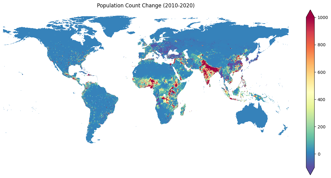
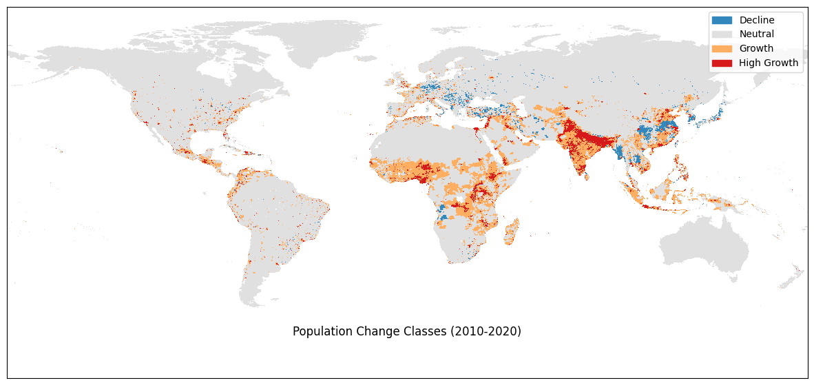
This is a good visualization, but not easy to interpret. Let’s create a better map with 4 discrete categories:

• Negative: Negative Cange upto -100.

• Neutral: Insignificant Negative or Positive Change between -100 to +100

• Growth: Small Positive Change between 100 to 1000.

• High Growth: Large Positive Change greater than 1000.

We use XArray Spatial’s reclassify() method to perform the reclassification from continuous values to 4 discrete classes.

class_bins = [-100, 100, 1000, np.inf]
class_values = [1, 2, 3, 4]
change_class = xrspatial.classify.reclassify(
    change.sel(band=1), bins=class_bins, new_values=class_values)

The result is a 2D array of reclassified values. We can visualize it the same way as before.

Since we have discrete pixel values, we can assign a specific color to each class using the levels parameter. The levels list defines the boundary of each interval and the colors list defines the colors assigned to each interval.

• Interval 1: Values between 1 and 2 (Decline)

• Interval 2: Values between 2 and 3 (Neutral)

• Interval 3: Values between 3 and 4 (Growth)

• Interval 4: Values between 4 and 5 (High Growth)

The imshow method supports only a colorbar legend which is not appropriate for a discrete classified raster such as ours. We use Matplotlib’s Patch() method to create a patch with appropriate labels and colors as described in Matplotlib’s Legend guide.

fig, ax = plt.subplots(1,1)
fig.set_size_inches(15,7)

levels = np.linspace(
    min(class_values), max(class_values) + 1, len(class_values) + 1)

colors = ['#3288bd', '#e0e0e0', '#fdae61', '#d7191c']
labels = ['Decline', 'Neutral', 'Growth', 'High Growth']

change_class.plot.imshow(
    ax=ax,
    add_colorbar=False,
    levels=levels,
    vmin=1,
    colors=colors)


patches =[mpatches.Patch(color=colors[i], label=labels[i]) for i in range(4)]
ax.legend(handles=patches)
ax.set_title('Population Change Classes (2010-2020)', y=0.1)

# Set axis labels off
ax.get_xaxis().set_visible(False)
ax.get_yaxis().set_visible(False)

plt.show()

Last step is to save the results to disk as a GeoTiff file.

output_file = 'change_class.tif'
output_file_path = os.path.join(output_folder, output_file)
change_class.rio.to_raster(output_file_path, compress='LZW')

---

If you want to give feedback or share your experience with this tutorial, please comment below. (requires GitHub account)