Calculating Standardized Precipitation Index (SPI)

Overview

One of the key advantages of the XEE package is the ability to use Python packages to work with data from Google Earth Engine. This package allows you to easily extract data from the vast data catalog of GEE and use widely used implementations available as Python libraries. This notebook shows how to extract a precipitation time-series images from Earth Engine and then use the Climate Indicies Python package to calculate the Calculating Standardized Precipitation (SPI).

Setup and Data Download

The following blocks of code will install the required packages and download the datasets to your Colab environment.

%%capture
if 'google.colab' in str(get_ipython()):
    !pip install climate-indices xee rioxarray

import ee
import xarray as xr
import rioxarray as rxr
import climate_indices
from climate_indices import indices
import matplotlib.pyplot as plt
import geopandas as gpd
import os
import datetime
import numpy as np

data_folder = 'data'
output_folder = 'output'

if not os.path.exists(data_folder):
    os.mkdir(data_folder)
if not os.path.exists(output_folder):
    os.mkdir(output_folder)

def download(url):
    filename = os.path.join(data_folder, os.path.basename(url))
    if not os.path.exists(filename):
        from urllib.request import urlretrieve
        local, _ = urlretrieve(url, filename)
        print('Downloaded ' + local)

data_url = 'https://naciscdn.org/naturalearth/10m/cultural/'


shapefile = 'ne_10m_admin_0_countries_ind.zip'

download(data_url + shapefile)

Initialize EE with the High-Volume EndPoint recommended to be used with XEE.

cloud_project = 'spatialthoughts'

try:
    ee.Initialize(
        project=cloud_project, 
        opt_url='https://earthengine-highvolume.googleapis.com'
    )
except:
    ee.Authenticate()
    ee.Initialize(
        project=cloud_project, 
        opt_url='https://earthengine-highvolume.googleapis.com'
    )

Procedure

Load the Natural Earth Admin0 boundaries and extract the polygon for India.

shapefile_path = os.path.join(data_folder, shapefile)
gdf = gpd.read_file(shapefile_path, encoding='utf-8')
country = gdf[gdf['SOV_A3'] == 'IND']

Now we have an ImageCollection that we want to get it as a XArray Dataset. We define the region of interest and extract the ImageCollection using the ‘ee’ engine.

era5 = ee.ImageCollection('ECMWF/ERA5_LAND/MONTHLY_AGGR')
filtered = era5 \
  .filter(ee.Filter.date('2000-01-01', '2025-01-01')) \
  .select('total_precipitation_sum')

geometry = country.geometry.union_all()
bounds = geometry.bounds

ds = xr.open_dataset(
    filtered,
    engine='ee',
    projection=filtered.first().select(0).projection(),
    geometry=bounds
)

The result is a XArray Dataset containing the image time-series.

ds

Select the total_precipitation_sum variable. Many XArray functions require all the dimensions to be sorted in ascending order. Make sure lat and lon are sorted.

da = ds.total_precipitation_sum
da = da.sortby(['lat', 'lon'])
da = da.fillna(0.0)
da

We now have a monthly precipitation time-series at each pixel. We can reformat the DataArray by grouping the time-series at each lat/lon.

da_precip_groupby = da.stack(pixel=('lat', 'lon')).groupby('pixel')

Configure the SPI calculation.

scale = 3
distribution = climate_indices.indices.Distribution.gamma
data_start_year = 2000
calibration_year_initial = 2000
calibration_year_final = 2024
periodicity = climate_indices.compute.Periodicity.monthly

def calculate_spi(group):
    spi_values = climate_indices.indices.spi(
        group.values,
        scale,
        distribution,
        data_start_year,
        calibration_year_initial,
        calibration_year_final,
        periodicity
    )
    return xr.DataArray(spi_values, coords={'time': group.time}, dims=['time'])

%%time
# apply SPI to each `pixel`
da_spi = da_precip_groupby.apply(calculate_spi)

Unstack the array back into original dimensions.

da_spi = da_spi.unstack('pixel')

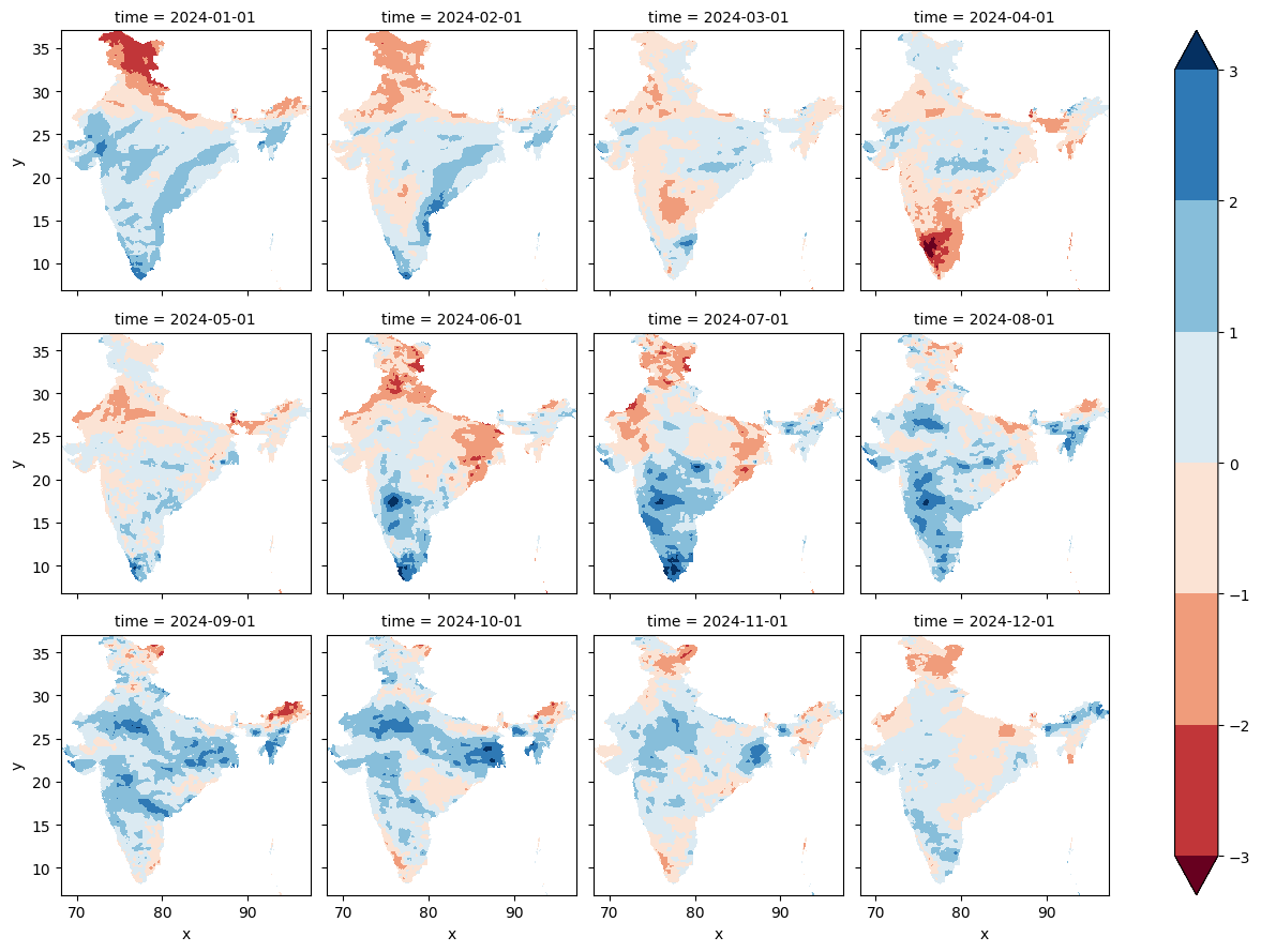
Visualize the Results

We use a faceted plot to visualize all months of a selected year.

# select a year to visualize
selected = da_spi.sel(time='2024')

legend_levels = [-3,-2,-1,0,1,2,3]
selected.plot(cmap='RdBu', col='time', col_wrap=4, levels=legend_levels)
plt.show()

Save Output as GeoTIFFs

We can use rioxarray to clip and save the resulting arrays as GeoTIFF files.

# select a year to save
selected = da_spi.sel(time='2024')

for time in selected.time.values:
    date_string = np.datetime_as_string(time, unit='M')
    image = selected.sel(time=time) \
      .rename({'lat': 'y', 'lon': 'x'}) \
      .transpose('y', 'x') \
      .rio.write_crs('EPSG:4326') \
      .rio.clip(country.geometry.values)
    output_file = f'{date_string}.tif'
    output_path = os.path.join(output_folder, output_file)
    image.rio.to_raster(output_path, driver='COG')
    print(f'Saved {output_path}')

---

If you want to give feedback or share your experience with this tutorial, please comment below. (requires GitHub account)