Extracting Time Series at Multiple Points with Xarray

Introduction

This notebook shows how to use XArray to efficiently extract a time-series at multiple coordinates. You will also learn how to use XArray to construct a datacube from individual cloud-hosted files and sample data from it with minimal data transfer.

Overview of the Task

We will take 12 individual Cloud-Optimized GeoTIFF (COG) files representing Soil Moisture for each month of a year, create a XArray Dataset from it and extract the soil moisture values for each month at multiple different locations.

Input Layers:

• soil_moisture_202301.tif, soil_moisture_202302.tif …: Cloud-Optimized GeoTIFF files representing average soil misture for each month. This files were exported from TerraClimate data hosted on Google Earth Engine using. See reference script

Output:

• soil_moisture.csv: A CSV file containing extracted monthly soil moisture values at 3 different coordinates.

Data Credit:

• Abatzoglou, J.T., S.Z. Dobrowski, S.A. Parks, K.C. Hegewisch, 2018, Terraclimate, a high-resolution global dataset of monthly climate and climatic water balance from 1958-2015, Scientific Data 5:170191, doi:10.1038/sdata.2017.191

Setup and Data Download

The following blocks of code will install the required packages and download the datasets to your Colab environment.

%%capture
if 'google.colab' in str(get_ipython()):
    !pip install rioxarray

import datetime
import glob
import os
import re
import matplotlib.pyplot as plt
import numpy as np
import pandas as pd
import geopandas as gpd
import xarray as xr
import rioxarray as rxr
import zipfile

data_folder = 'data'
output_folder = 'output'

if not os.path.exists(data_folder):
    os.mkdir(data_folder)
if not os.path.exists(output_folder):
    os.mkdir(output_folder)

Data Pre-Processing

In this example, we have a folder on Google Cloud Storage (GCS) has 12 Cloud-Optomized GeoTIFF files representing soil moisture for each month. The file URIs are as below

gs://spatialthoughts-public-data/terraclimate/soil_moisture_202301.tif
gs://spatialthoughts-public-data/terraclimate/soil_moisture_202302.tif
gs://spatialthoughts-public-data/terraclimate/soil_moisture_202303.tif
...

First we create an XArray Dataset from these individual files.

The files will be read using the GDAL library which allows reading cloud-hosted files directly. Files on Google Cloud Storage can be read using the /vsigs/ prefix. Since our files are public, we specify the GS_NO_SIGN_REQUEST=YES option. For accessing data on private bucket, see the authentication options specified in GDAL and Google Cloud Storage (GCS) .

os.environ['GS_NO_SIGN_REQUEST'] = 'YES'
prefix = '/vsigs/spatialthoughts-public-data/terraclimate/'

# Create a list of URIs with /vgigs/ prefix
urls = []
for month in range(1, 13):
    image_id = f'soil_moisture_2023{month:02d}.tif'
    path = prefix + image_id
    urls.append(path)

urls

def path_to_datetimeindex(filepath):
  filename = os.path.basename(filepath)
  pattern = r'soil_moisture_(\d+).tif'
  match = re.search(pattern, filepath)
  if match:
      doy_value = match.group(1)
      timestamp = datetime.datetime.strptime(doy_value, '%Y%m')
      return timestamp
  else:
    print('Could not extract DOY from filename', filename)


timestamps = []
filepaths = []

for filepath in urls:
  timestamp = path_to_datetimeindex(filepath)
  filepaths.append(filepath)
  timestamps.append(timestamp)

unique_timestamps = sorted(set(timestamps))

scenes = []

for timestamp in unique_timestamps:
  filename = f'soil_moisture_{timestamp.strftime('%Y%m')}.tif'
  filepath = prefix + filename
  print(f'Reading {filepath}')
  scene = rxr.open_rasterio(filepath, chunks={'x':512, 'y':512})
  scenes.append(scene)

time_var = xr.Variable('time', list(unique_timestamps))

time_series_scenes = xr.concat(scenes, dim=time_var)
time_series_scenes

<xarray.DataArray (time: 12, band: 1, y: 4321, x: 8641)> Size: 4GB
dask.array<concatenate, shape=(12, 1, 4321, 8641), dtype=float64, chunksize=(1, 1, 512, 512), chunktype=numpy.ndarray>
Coordinates:
  * time         (time) datetime64[ns] 96B 2023-01-01 2023-02-01 ... 2023-12-01
  * band         (band) int64 8B 1
  * y            (y) float64 35kB 89.98 89.94 89.9 ... -89.94 -89.98 -90.02
  * x            (x) float64 69kB -180.0 -179.9 -179.9 ... 179.9 180.0 180.0
    spatial_ref  int64 8B 0
Attributes:
    AREA_OR_POINT:  Area
    scale_factor:   1.0
    add_offset:     0.0
    long_name:      soil

xarray.DataArray

• time: 12
• band: 1
• y: 4321
• x: 8641

• dask.array<chunksize=(1, 1, 512, 512), meta=np.ndarray>

  Array Chunk Bytes 3.34 GiB 2.00 MiB Shape (12, 1, 4321, 8641) (1, 1, 512, 512) Dask graph 1836 chunks in 37 graph layers Data type float64 numpy.ndarray

• Coordinates: (5)
  • time
    (time)
    datetime64[ns]
    2023-01-01 ... 2023-12-01

    array(['2023-01-01T00:00:00.000000000', '2023-02-01T00:00:00.000000000',
           '2023-03-01T00:00:00.000000000', '2023-04-01T00:00:00.000000000',
           '2023-05-01T00:00:00.000000000', '2023-06-01T00:00:00.000000000',
           '2023-07-01T00:00:00.000000000', '2023-08-01T00:00:00.000000000',
           '2023-09-01T00:00:00.000000000', '2023-10-01T00:00:00.000000000',
           '2023-11-01T00:00:00.000000000', '2023-12-01T00:00:00.000000000'],
          dtype='datetime64[ns]')

  • band
    (band)
    int64
    1

    array([1])

  • y
    (y)
    float64
    89.98 89.94 89.9 ... -89.98 -90.02

    array([ 89.979167,  89.9375  ,  89.895833, ..., -89.9375  , -89.979167,
           -90.020833])

  • x
    (x)
    float64
    -180.0 -179.9 ... 180.0 180.0

    array([-179.979167, -179.9375  , -179.895833, ...,  179.9375  ,  179.979167,
            180.020833])

  • spatial_ref
    ()
    int64
    0

    crs_wkt :

    GEOGCS["unknown",DATUM["unknown",SPHEROID["Spheroid",6378137,298.257223563]],PRIMEM["Greenwich",0],UNIT["degree",0.0174532925199433,AUTHORITY["EPSG","9122"]],AXIS["Latitude",NORTH],AXIS["Longitude",EAST]]

    semi_major_axis :

    6378137.0

    semi_minor_axis :

    6356752.314245179

    inverse_flattening :

    298.257223563

    reference_ellipsoid_name :

    Spheroid

    longitude_of_prime_meridian :

    0.0

    prime_meridian_name :

    Greenwich

    geographic_crs_name :

    unknown

    horizontal_datum_name :

    unknown

    grid_mapping_name :

    latitude_longitude

    spatial_ref :

    GEOGCS["unknown",DATUM["unknown",SPHEROID["Spheroid",6378137,298.257223563]],PRIMEM["Greenwich",0],UNIT["degree",0.0174532925199433,AUTHORITY["EPSG","9122"]],AXIS["Latitude",NORTH],AXIS["Longitude",EAST]]

    GeoTransform :

    -180.0 0.041666666666666664 0.0 90.0 0.0 -0.041666666666666664

    array(0)

• Attributes: (4)

  AREA_OR_POINT :

  Area

  scale_factor :

  1.0

  add_offset :

  0.0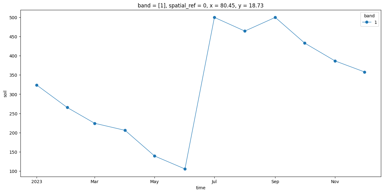

  long_name :

  soil

Plotting the time-series

We extract the time-series at a specific X,Y coordinate.

time_series = time_series_scenes.interp(x=80.449, y=18.728)

fig, ax = plt.subplots(1, 1)

fig.set_size_inches(15, 7)
time_series.plot.line(ax=ax, x='time', marker='o', linestyle='-', linewidth=1)
plt.show()

Extracting Time-Series at Multiple Locations

locations = [
    ('Location 1', 80.449, 18.728),
    ('Location 2', 79.1488, 15.2797),
    ('Location 3', 74.656, 25.144)
]

df = pd.DataFrame(locations, columns=['Name', 'x', 'y'])
geometry = gpd.points_from_xy(df.x, df.y)
gdf = gpd.GeoDataFrame(df, crs='EPSG:4326', geometry=geometry)
gdf

	Name	x	y	geometry
0	Location 1	80.4490	18.7280	POINT (80.449 18.728)
1	Location 2	79.1488	15.2797	POINT (79.1488 15.2797)
2	Location 3	74.6560	25.1440	POINT (74.656 25.144)

x_coords = gdf.geometry.x.to_xarray()
y_coords = gdf.geometry.y.to_xarray()

sampled = time_series_scenes.sel(x=x_coords, y=y_coords, method='nearest')

Convert the sampled dataset to a Pandas Series.

sampled_df = sampled.to_series()
sampled_df.name = 'soil_moisture'
sampled_df = sampled_df.reset_index()
sampled_df.head()

	time	band	index	soil_moisture
0	2023-01-01	1	0	322.5
1	2023-01-01	1	1	33.5
2	2023-01-01	1	2	25.1
3	2023-02-01	1	0	264.4
4	2023-02-01	1	1	26.4

Add a formatted time column

sampled_df['formatted_time'] = sampled_df['time'].dt.strftime("%Y_%m")
sampled_df.head()

	time	band	index	soil_moisture	formatted_time
0	2023-01-01	1	0	322.5	2023_01
1	2023-01-01	1	1	33.5	2023_01
2	2023-01-01	1	2	25.1	2023_01
3	2023-02-01	1	0	264.4	2023_02
4	2023-02-01	1	1	26.4	2023_02

Convert this to a wide table, with each month’s value as a column.

wide_df = sampled_df.pivot(index='index', columns='formatted_time', values='soil_moisture')
wide_df = wide_df.reset_index()
wide_df.iloc[:, :10]

formatted_time	index	2023_01	2023_02	2023_03	2023_04	2023_05	2023_06	2023_07	2023_08	2023_09
0	0	322.5	264.4	223.0	204.8	138.1	104.7	498.9	462.5	498.9
1	1	33.5	26.4	21.8	18.7	16.3	14.5	125.6	51.1	67.2
2	2	25.1	21.2	18.4	16.3	14.6	13.7	34.6	27.5	37.7

Merge the extracted value with the original data.

merged = pd.merge(gdf, wide_df, left_index=True, right_index=True)
merged.iloc[:, :10]

	Name	x	y	geometry	index	2023_01	2023_02	2023_03	2023_04	2023_05
0	Location 1	80.4490	18.7280	POINT (80.449 18.728)	0	322.5	264.4	223.0	204.8	138.1
1	Location 2	79.1488	15.2797	POINT (79.1488 15.2797)	1	33.5	26.4	21.8	18.7	16.3
2	Location 3	74.6560	25.1440	POINT (74.656 25.144)	2	25.1	21.2	18.4	16.3	14.6

Finally, we save the sampled result to disk as a CSV.

output_filename = 'soil_moisture.csv'
output_path = os.path.join(output_folder, output_filename)
output_df = merged.drop(columns=['geometry', 'index'])
output_df.to_csv(output_path, index=False)

---

If you want to give feedback or share your experience with this tutorial, please comment below. (requires GitHub account)